Overview
COMP110, like all things, must come to an end. We are sad, too. For you, though, your programming journey is just beginning! In this project, you will gain practice using Pandas, a real world, industrial grade data analysis library. You will be expected to peruse official tutorials and documentation to figure out how to perform data exploration and analysis.
After COMP110, when you are on your own and would like to take on a new programming project, we hope you will think back to the experience you are about to have with this project and in Lesson 26. The process we are guiding you through here is applicable to learning most any other programming language, library, or software-driven technology. If you want to make a game, an app, a web site, and so on, the same strategies directly apply!
Before beginning this project you must fully complete Lesson 26 - Guided Readings on NumPy and Pandas. While we could easily teach these same concepts in COMP110-specific videos, as with earlier topics, here we are intentionally setting you off in the direction of public, official, free documentation. Not only will this help you know what to expect from library and programming tool websites, but it will also give you confidence you can learn new skills and technologies outside of formal instruction!
Data Set
We will use a data set sourced from the World Bank. It is a CSV file that contains many data points most related to education, referred to as indicators, for countries around the world in 2018. Not all all countries have data on all indicators, some are blank. The World Bank’s Data Bank has lots of data beyond this, at global and local scales, and across much wider time frames.
SP.POP.1564.TO.ZS- Population ages 15-64 (% of total population)SP.POP.0014.TO.ZS- Population ages 0-14 (% of total population)SL.UEM.TOTL.ZS- Unemployment, total (% of total labor force) (modeled ILO estimate)SL.UEM.TOTL.MA.ZS- Unemployment, male (% of male labor force) (modeled ILO estimate)SL.UEM.TOTL.FE.ZS- Unemployment, female (% of female labor force) (modeled ILO estimate)SL.TLF.TOTL.IN- Labor force, totalSL.TLF.TOTL.FE.ZS- Labor force, female (% of total labor force)SH.DYN.2024- Probability of dying among youth ages 20-24 years (per 1,000)SH.DYN.1519- Probability of dying among adolescents ages 15-19 years (per 1,000)SH.DYN.1014- Probability of dying among adolescents ages 10-14 years (per 1,000)SH.DYN.0509- Probability of dying among children ages 5-9 years (per 1,000)SH.DTH.2024- Number of deaths ages 20-24 yearsSH.DTH.1519- Number of deaths ages 15-19 yearsSH.DTH.1014- Number of deaths ages 10-14 yearsSH.DTH.0509- Number of deaths ages 5-9 yearsSE.XPD.TOTL.GD.ZS- Government expenditure on education, total (% of GDP)SE.XPD.TOTL.GB.ZS- Government expenditure on education, total (% of government expenditure)SE.TER.ENRR.MA- School enrollment, tertiary, male (% gross)SE.TER.ENRR.FE- School enrollment, tertiary, female (% gross)SE.TER.ENRR- School enrollment, tertiary (% gross)SE.SEC.TCHR.FE.ZS- Secondary education, teachers (% female)SE.SEC.TCHR.FE- Secondary education, teachers, femaleSE.SEC.TCHR- Secondary education, teachersSE.SEC.PRIV.ZS- School enrollment, secondary, private (% of total secondary)SE.SEC.NENR.MA- School enrollment, secondary, male (% net)SE.SEC.NENR.FE- School enrollment, secondary, female (% net)SE.SEC.NENR- School enrollment, secondary (% net)SE.SEC.ENRR.MA- School enrollment, secondary, male (% gross)SE.SEC.ENRR.FE- School enrollment, secondary, female (% gross)SE.SEC.ENRR- School enrollment, secondary (% gross)SE.SEC.ENRL.VO.FE.ZS- Secondary education, vocational pupils (% female)SE.SEC.ENRL.VO- Secondary education, vocational pupilsSE.SEC.ENRL.TC.ZS- Pupil-teacher ratio, secondarySE.SEC.ENRL.LO.TC.ZS- Pupil-teacher ratio, lower secondarySE.SEC.ENRL.GC.FE.ZS- Secondary education, general pupils (% female)SE.SEC.ENRL.GC- Secondary education, general pupilsSE.SEC.ENRL.FE.ZS- Secondary education, pupils (% female)SE.SEC.ENRL- Secondary education, pupilsSE.SEC.DURS- Secondary education, duration (years)SE.SEC.CMPT.LO.ZS- Lower secondary completion rate, total (% of relevant age group)SE.SEC.CMPT.LO.MA.ZS- Lower secondary completion rate, male (% of relevant age group)SE.SEC.CMPT.LO.FE.ZS- Lower secondary completion rate, female (% of relevant age group)SE.SEC.AGES- Lower secondary school starting age (years)SE.PRM.UNER.ZS- Children out of school (% of primary school age)SE.PRM.UNER.MA.ZS- Children out of school, male (% of male primary school age)SE.PRM.UNER.MA- Children out of school, primary, maleSE.PRM.UNER.FE.ZS- Children out of school, female (% of female primary school age)SE.PRM.UNER.FE- Children out of school, primary, femaleSE.PRM.UNER- Children out of school, primarySE.PRM.TENR- Adjusted net enrollment rate, primary (% of primary school age children)SE.PRM.TCHR.FE.ZS- Primary education, teachers (% female)SE.PRM.TCHR- Primary education, teachersSE.PRM.REPT.ZS- Repeaters, primary, total (% of total enrollment)SE.PRM.REPT.MA.ZS- Repeaters, primary, male (% of male enrollment)SE.PRM.REPT.FE.ZS- Repeaters, primary, female (% of female enrollment)SE.PRM.PRSL.ZS- Persistence to last grade of primary, total (% of cohort)SE.PRM.PRSL.MA.ZS- Persistence to last grade of primary, male (% of cohort)SE.PRM.PRSL.FE.ZS- Persistence to last grade of primary, female (% of cohort)SE.PRM.PRIV.ZS- School enrollment, primary, private (% of total primary)SE.PRM.OENR.ZS- Over-age students, primary (% of enrollment)SE.PRM.OENR.MA.ZS- Over-age students, primary, male (% of male enrollment)SE.PRM.OENR.FE.ZS- Over-age students, primary, female (% of female enrollment)SE.PRM.NENR- School enrollment, primary (% net)SE.PRM.GINT.ZS- Gross intake ratio in first grade of primary education, total (% of relevant age group)SE.PRM.GINT.MA.ZS- Gross intake ratio in first grade of primary education, male (% of relevant age group)SE.PRM.GINT.FE.ZS- Gross intake ratio in first grade of primary education, female (% of relevant age group)SE.PRM.ENRR.MA- School enrollment, primary, male (% gross)SE.PRM.ENRR.FE- School enrollment, primary, female (% gross)SE.PRM.ENRR- School enrollment, primary (% gross)SE.PRM.ENRL.TC.ZS- Pupil-teacher ratio, primarySE.PRM.ENRL.FE.ZS- Primary education, pupils (% female)SE.PRM.ENRL- Primary education, pupilsSE.PRM.DURS- Primary education, duration (years)SE.PRM.CMPT.ZS- Primary completion rate, total (% of relevant age group)SE.PRM.CMPT.MA.ZS- Primary completion rate, male (% of relevant age group)SE.PRM.CMPT.FE.ZS- Primary completion rate, female (% of relevant age group)SE.PRM.AGES- Primary school starting age (years)SE.PRE.ENRR.MA- School enrollment, preprimary, male (% gross)SE.PRE.ENRR.FE- School enrollment, preprimary, female (% gross)SE.PRE.ENRR- School enrollment, preprimary (% gross)SE.PRE.ENRL.TC.ZS- Pupil-teacher ratio, preprimarySE.PRE.DURS- Preprimary education, duration (years)SE.ENR.TERT.FM.ZS- School enrollment, tertiary (gross), gender parity index (GPI)SE.ENR.SECO.FM.ZS- School enrollment, secondary (gross), gender parity index (GPI)SE.ENR.PRSC.FM.ZS- School enrollment, primary and secondary (gross), gender parity index (GPI)SE.ENR.PRIM.FM.ZS- School enrollment, primary (gross), gender parity index (GPI)SE.COM.DURS- Compulsory education, duration (years)
For a more thorough description of any indicator, use the WorldBank’s Metadata Glossary to search for the indicator.
Your goal in this project is to choose two indicators from the above options, state a hypothesis as to whether there is a strong or weak correlation between the two factors, and perform various analysis as described below to investigate.
Getting Started
To get the data for the project, right click this link in Google Chrome and select “Save Link As…”. Download the file to your course workspace’s data directory in a file named databank_education_2018.csv.
In your course workspace, create a new directory in projects called pj02.
In your projects/pj02 directory, create a new notebook titled analysis.ipynb.
Begin your Jupyter Notebook with a markdown cell that describes your hypothesis about the two indicators you are investigating.
Add a code cell that imports the pandas library in a conventional way, aliasing it as pd.
In the same code cell as above, declare and initialize two named constants for each of the indicator code strings you will explore. Name these with more descriptive names than the codes themselves to help make your notebook more readable.
Requirements
Each of these requirements can be completed in its own code cell. Above each code cell, you must have a markdown cell that describes in plain, well-written English what is about to follow.
0. Read the CSV file into a DataFrame. The str path you will need to use with Pandas’ read_csv function is:
"../../data/databank_education_2018.csv"The two sets of .. refer to “moving up” two directories (from pj02 -> projects -> workspace) and then into the data directory where you downloaded the CSV.
1. Shape and Head
After reading the CSV file into a DataFrame, print the shape of the DataFrame (rows, columns). Then, use the head method of DataFrame to display the first 10 rows.
2. Selecting Column Subsets
Use column-based selection to narrow in on a DataFrame with only the three columns your analysis is concerned with: "Country" and the two indicator columns you choose and assigned to named constants in Getting Started. Once again, use the head method to display the first 10 rows of your selection.
3. Selecting Rows with Complete Data
Use row-based filtering to select only rows where neither of your analysis columns have N/A or NaN (Not a Number) values. Print the shape of the resulting DataFrame and notice how many fewer rows there are than the complete dataset. Complete the cell with a method call expression to head to display the first 10 rows of your narrowed data set. You should see values for each row and column.
Hint: Recall from the guided reading that a column/Series has a built-in notna method. Also recall the note that you can combine by and’ing two bool Serieses with the & operation.
4. 10-largest Values
Choose either of your indicator columns and sort its values in descending order (hint: search for DataFrame sort_values and look for an examples – note that this method does not mutate the original DataFrame and returns a new DataFrame, instead). Use head to display the rows with the 10 largest values in the column you choose in descending order.
5. Scatter Plot
Produce a Scatter Plot where one of your indicator columns serves as the X-axis and the other as the Y-axis. See the official Pandas getting started tutorial on plotting for help getting started.
6. Correlation
Every Pandas Series object (each column) has the ability to compute a linear correlation with another Series of the same length. Search around for documentation for how to use a Series’s method for correlating it with some other Series object. Print the correlation between your two indicator columns. The exact details of correlation are beyond the scope of COMP110, but the closer to 0 a correlation is, the less correlated two indicators are. Conversely, the closer to 1 or -1 the stronger the correlation is between two indicators. A strong, positive correlation suggests as one indicator increases, so does the other. A strong, negative correlation suggests as one indicator increases, the other decreases. When thinking about correlation, know that correlation is not causation and a strong relationship between two variables does not imply one causes the other nor vice-versa.
Rubric
Reporting – 30 points
- 10 points - First markdown cell in your notebook states your hypothesis or question of interest
- 10 points - Each cell of code that you write must be preceeded by a markdown cell explaining what you are attempting to do. Walk us through your thought process.
- 10 points - Final markdown cell is a conclusion paragraph summarizing your findings. Were you able to answer your question or prove your hypothesis? It is totally OK (and part of the process) to not get what you initially expected. You can still get full credit even if you end up contradicting your hypothesis :)
Markdown tip! If you want to make something a big header, you can start the line with # for a big header, ## for a medium header, ### for a small one.
Analysis – 60 points
- 10 points - Establishing and using named constants rather than indicator codes
- 10 points each - Requirements 2 through 6 above
Above and Beyond Charting – 10 points (from A- to A)
The UTAs cannot help you with these final 10 points. These are practice (and reward) for learning how to search and tinker around with your code in order to achieve an outcome. You are allowed to Google and use resources you find, but collaboration is still prohibited.
- 5 points - Label the axes of your chart more meaningfully than the indicator codes and give it a title.
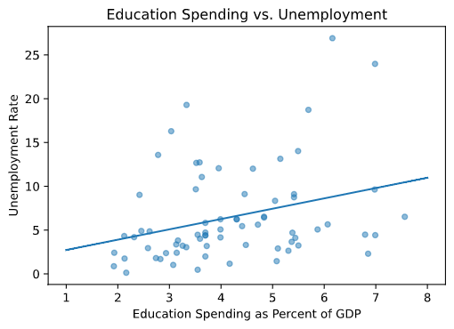
- 5 points - Challenging: Compute and plot a regression line on your scatter plot using
numpy. You may want to search around for functions including:polyfit,poly1d,linspace, andpolyval. An example plot with a regression line is shown below:
Submission Instructions
Run python -m tools.submission projects/pj02 to build your submission zip for upload to Gradescope. Don’t forget to backup your work by creating a commit and pushing it to GitHub. For a reminder of this process, see the previous exercises.
All of the points for this project will be handgraded, so your autograder score should be 0/0. This blank screen is expected!